Lukas Rieder, Author at Management Control: Blog and Downloads

Localize Cost Reduction Potentials

When actual data is available to measure realized cost reductions, it is too late! In the meantime, the competition has already acted, which may have resulted in shifts in market share that give faster growing companies better opportunities for cost reductions than to one’s own company. Consequently, cost reduction potentials must be actively sought, planned and implemented.

Improving the cost position requires creative, innovative ideas. Realizing cost reductions means strenuous operational work.

Localize Cost Reduction Potentials

It is important to remember that effectiveness (scope and impact) comes before efficiency (less input for more output).

Giving regular feedback to one’s own employees on the performance and quality achieved increases effectiveness because the people being managed can thus control and improve their own efforts (see the post “Master Plan for Integrated Planning and Control”).

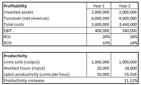
In order to be able to localize and realize cost reduction potentials, many methods and procedures have already been developed and recommended. The intention is to reduce costs or to let them grow slower than the realized net revenues, thus generating profits that can be used for the expansion of the organization.

Some proven successful methods and tools are listed below together with the improvements hoped for by their application.

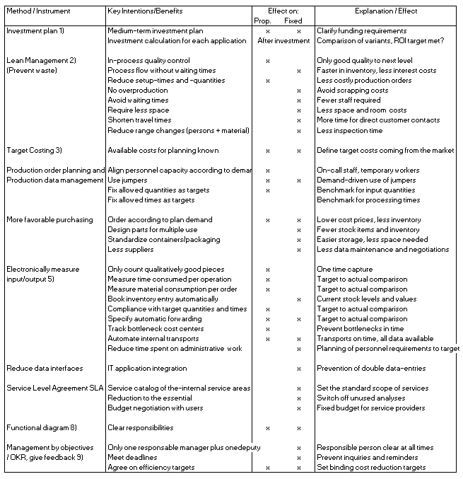
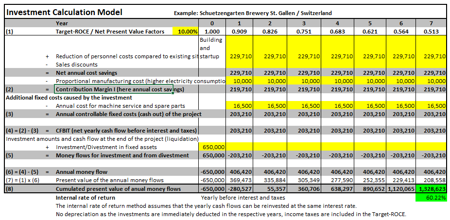
1 Strategy and investment planning see the capital budgeting Excel-download

2 Lean management

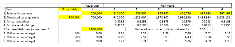
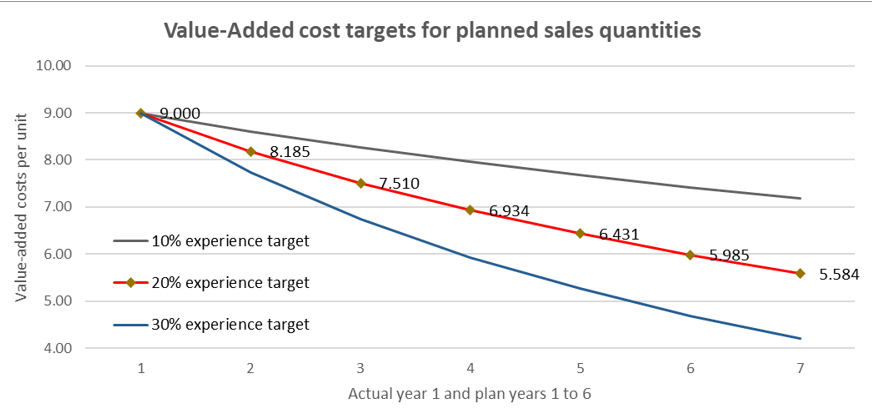
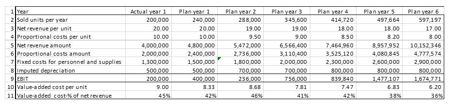
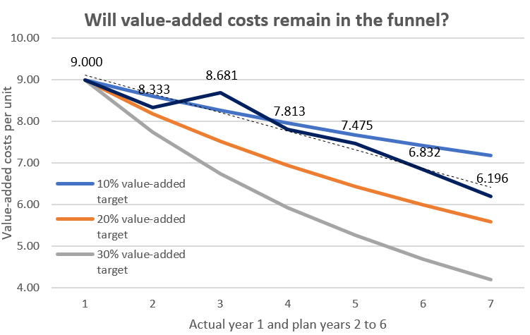
3 Target costing: In simplified terms, target costing is intended to bring the expected future market into product development and production, thereby piloting a strong cost position as early as in the product design stage. A target cost calculation is used to determine the maximum costs that can be incurred for manufacturing the product, based on the net revenue that can be achieved on the market. The current percentages for the share of administrative and sales costs and for the target profit are deducted from the net revenue (estimation of a target contribution margin for these functions). The amount available for producing the planned quantities remains as the residual. For the quantification of the various items, dynamic investment appraisal must again be used, since target costing decisions usually require investments to be taken into account and implementation often takes several years.

4 Production data management

5 Measure input/output electronically

6 Plan and record internal tasks

7 Service Level Agreements (SLA) This is a service agreement between clients (internal divisions, functions and cost centers) and performing cost centers for the regulation of recurring services. An SLA is often also agreed with external service providers (e.g., IT outsourcing).

The purpose of such a service agreement is to describe the services to be provided by the service provider as completely as possible for the contractual partners. Care must be taken to ensure that the services are defined in such a way that they can be measured or at least verified.

In the SLA, the contractor is one or more cost centers; the customer is the community of cost centers receiving the services.

The supplier (cost center manager) is responsible for the service provision and for the target cost compliance. Therefore, he also has the obligation to say no if (in the plan or in the actual) more than what has been agreed is demanded. In return, the clients are responsible for approving the budget for the specified services. If they want more service or to pay less, the service providers can reject the proposed conditions. This agreement work must be fixed as part of the budgeting process. After all, once the authorizations are in place, the staff is hired and the money is spent.

Services provided by internal functions are often very diverse and can only be predicted imprecisely. This makes it difficult to agree on an SLA. Nevertheless, it is worthwhile for both contracting parties to describe the work to be performed as completely and comprehensibly as possible. After all, these minutes are an important element for budgeting and comparing planned/actual data. The following should be specified for each item

- Quantity: e.g., preparation of a monthly financial statement or ensuring 99% availability of applications.
- Quality: e.g., according to the principles of proper accounting or the response times of the systems to be maintained.
- Deadlines: e.g., on the 5th working day of the following month or response time until faults are resolved (service level).
- Costs / results: budget compliance.

The tasks to be performed in an SLA should be limited to what is necessary. As a result, the cost of SLA fulfillment should increase more slowly than the CM-volume of the company.

When an SLA is released, contractors may deploy their personnel and resources. The internal customers must periodically be given the opportunity to comment on the extent and quality of service delivery.

SLA costs are fixed costs. They are incurred for the using cost centers, not directly for the products. Due to the lack of a direct cause-effect relationship, they cannot be allocated to the products.

8 Functional diagram

Operational Excellence

Many brilliant strategic decisions have laid the foundation for exponential development of companies. Again, many of these companies have found their way into economic history as “success stories”. They are quoted in books and in seminars.

However, in the cases known to us, the fact that things got this far was always due to “operational excellence”. In our view, fine-tuning details, mastering processes, distinguishing between what is necessary and what is “good to have”, and continuously improving implementation are basic elements of successful corporate management, both in the area of sales and distribution and in the persistent improvement of the company’s own cost position.

Experience Curve for Your Company

How to develop the experience curve for the own company.

For the empirical proof of the experience curve, series of actual figures from various industries were used. These showed that the value-added costs per unit decreased by 20 – 30% for each doubling of the cumulative output quantity. This finding can also be used as a guideline for planning for one’s own company. Based on actual data (partly estimated), a company-specific experience curve can be drawn up. This can be used to analyze whether the medium-term planning figures will be suitable for implementing the experience curve in one’s own company.

Experience curve for Your company

The following initial data are required:

- Cumulative sales volume to date
- Value added costs of the most recent actual year
- Planned sales volumes for the planning horizon under consideration.

From this data, a “funnel”, i.e., a corridor for the development of the allowable value-added costs, can be calculated.

First, the annual context must be established (Compare with the table “calculation of cost reduction targets” below):

- In line 1, the actual sales volumes of year 1 and the planned sales volumes of the planning years 2-7 are entered.
- The sales volume of the assortment sold before year 1 is entered in line 2 (500,000 units). Since this is only a rough estimate, all product units are considered equal for simplicity. Also in line 2, the accumulated sales quantities until the end of the planning horizon are calculated.
- From this, the doublings per year can be calculated in line 3. The formula for this is:
  Formula to calculate annual doublings
  
  The fact that these values are continuously decreasing expresses that despite sales volume increases, an increasing number of years is needed to achieve another doubling.

- Line 4 shows the cumulative doublings of the planned years in relation to the initial situation. They form the basis for calculating the theoretical experience curve values.
- In line 5, the value added costs per unit of the actual year are calculated (1’800’000 : 200’000 sales volume = 9.00).
- Since a cumulative doubling of 0.4253 is to be achieved in planned sales in year 2 compared to actual year 1, the value-added costs of the previous year are exponentiated by the cumulative doubling factor (0.4253 in planned year 1). Depending on the selected experience curve target, this results in the value-added costs to be achieved in the respective plan year (e.g., 8.19 for the 20% experience curve for plan year 1, line 7).
- Purely arithmetically, the experience curves of 10%, 20% and 30% can be determined in lines 6-8 for the value-added costs per sales unit to be achieved.

Graphically, the “funnel” is created, in which the planned and effective value-added costs should move within the medium-term planning horizon shown (Plan1 to Plan 6).

Value-added cost targets for planned sales quantities

The next post will ask whether the medium-term cost center plans for the value-added cost areas will be able to meet these requirements. If not, ideas must be generated on how to reduce the planned costs of the affected cost centers. If this requirement cannot be met, the company will lose competitiveness due to excessively high value-added costs.

Importance of cumulative past sales volume

It is often difficult for companies to determine the cumulative sales volume to date, either because the data is missing or because estimates had to be made due to changes in the portfolio.

If, in the model presented above, the cumulative past sales volume is entered as 0 units, the value-added costs to be achieved per unit sold in plan year 1 and assuming an experience curve target of 20% will decrease from 8.19 to 6.49 per unit. In the opposite case, where the cumulative sales volume to date is 1,000,000 instead of 500,000 units, the allowable value-added costs increase to 8.49 per unit.

If these extreme variants are considered, it can be seen that an incorrectly estimated or calculated cumulative sales volume is significant, but the target values to be achieved change little. Overestimated cumulative past sales volumes lead to lower cost reduction targets for the planning years, while underestimated ones lead to higher ones. As these are planning targets, possible misestimates are justifiable.

Improve cost position

If you do not improve your cost position, your competition can overtake you.

Part of the consumer experience is that products, ignoring price changes due to inflation, are offered cheaper per unit over time, or that greater performance is offered for the same price.

Some examples:

In 1983, the Motorola Dyna Tac 8000x became the first commercially offered cell phone to hit the market at $3,995. Thirty years later, a cell phone with more features and no ties to a service provider can be purchased at a specialty retailer for about $20, or roughly 5‰.

The original IBM personal computer was introduced to the market in 1981 at a price of $1,565. Thirty years later, PCs were available for purchase for well under $100. These were also much more powerful than the original and offered more features. The HP LaserJet printer hit the market in 1984 at a price of $3,495. After about 30 years, laser printers were on sale around $100.

In https://winhistory.de, the development of the sales prices per megabyte of hard disk capacity from 1997 to 2011 is shown:

The fact that more output is offered for the same price over time can be observed in many areas of the economy. The main reasons for this are technological improvements, competition, and rising production volumes.

Improve cost position

A company must continuously strive to reduce its average total cost per unit of output. If it does not manage to do this, its existing or new competitors will do so, worsening its market position as well as the sales opportunities of the company.

A rapidly and continuously improved cost position is therefore a key prerequisite for achieving or maintaining a strong market position. Companies must be able to substantially reduce their average per unit costs of goods over time if they want to parry sales price reductions by competitors and maintain their profitability. Some of the companies that have managed this balancing act have become global corporations. Many others had to give up because they were not able to reduce the cost per manufactured unit to a sufficient extent.

These relationships have been known for a long time. As a result of his empirical investigations, B.D. Henderson presented the law of experience – also known as the experience curve or Boston effect – as early as 1974 (cf. B.D. Henderson, die Erfahrungskurve in der Unternehmensstrategie, Frankfurt/New York, 1974).

In the following posts, the determinants of the experience curve are first analyzed. It is then shown how the concept of the experience curve can be integrated into one’s own planning and control. The focus is on the alignment of internal objectives with external market developments.

Promises of the experience curve

In every company ways have to be found to implement the experience curve.

Bruce Henderson (cf. B.D. Henderson, The Experience Curve, Boston Consulting Group, Perspectives nr. 16, 1968 ) has proven with extensive empirical studies (ex post) for entire industries or for the product volumes offered in a market in various industries that:

The real (inflation-adjusted) full value-added costs decrease by 20 to 30% with each doubling of cumulative output volume.

Promises of the experience curve

The practical application of this finding in one’s own organization requires that the statement be viewed in a differentiated manner:

- The cost reduction applies to every doubling of the cumulative output quantity (since the market launch of an offering). How quickly a doubling takes place consequently depends on the market and on the company’s own growth. In fast-growing markets, a doubling of the cumulative output quantity (of all suppliers) can take place in a few months; in mature markets, it may take several years.
- Value-added costs comprise the costs of the services provided within the company itself. These are primarily the total (proportional and fixed) personnel costs and the externally purchased services consumed, as well as depreciation and amortization (fixed costs only). They are incurred so that the company’s own services can be delivered and profit can be generated. Direct product-related material and external service costs are not part of the value-added costs, as these are determined by the suppliers. Value-added costs are calculated by deducting from total expenses in the income statement the material and external service consumption directly caused by the products sold.

The value-added costs per unit sold must be reduced if competitiveness is to be increased. The graph shows the development of the value-added costs for each doubling of cumulative output quantity, assuming that the items sold remain the same.

Value added and cost of goods sold per unit must be reduced based on experience.

- The absolute company profit increases as long as the sales price can be maintained (in the example at 12.00) and the value-added costs as well as the costs for material and external services can be reduced according to the doublings.
- However, the experience curve also applies to competitors. If they manage the doublings faster, they also have the chance to reduce their value-added costs per unit faster. This increases their potential to lower their net selling prices and thus improve their market position.
- The graph does not contain a calendar reference. Therefore, it is not yet possible to derive which cost reductions can be realized in which years. The corresponding procedure will be explained in a further post.

There are four factors that determine the realization of experience curve progress: economies of scale, learning effect, improved processes, and product design.

- Economies of scale occur more or less automatically. If the sales volume and thus the production volume increase, the fixed cost block is distributed over more units, which reduces the average complete product cost.
- People and machines learn from experience. Through repetition, consistent processes can be completed in less time. Processes become more efficient, resulting in lower processing times per unit. Administrative processes can also be completed with less time and fewer errors. Integrated data processing makes information available across departments, and machine learning and artificial intelligence can automate many evaluation tasks.
- By using new and more powerful equipment, manufacturing can be done with less time and possibly improved quality. Often, such investments are combined with capacity expansions.
- New materials and new designs enable more cost-effective manufacturing. Changes in product design should at the same time allow for higher sales volumes and changed sales prices.

Application example:

Development of prices, costs and EBIT over 7 years

The table and the graphs show by way of example how the experience curve factors and the increase in sales volumes over seven years affect earnings before interest and taxes (EBIT):

- The increase in sales volumes over the years leads to sharply rising net revenues per unit, despite falling net revenues.
- Fixed costs fall per unit, although the absolute amounts for depreciation and fixed personnel and material costs rise (fixed cost degression).
- Due to learning effects and process improvements in production as well as possibly due to more favorable material purchases, the proportional manufacturing costs decrease from 10.00 to 8.00 per unit.

The form of presentation of the changes selected above presupposes that in management accounting a clear distinction is made between proportional and fixed costs and that a contribution margin calculation is prepared (cf., the corresponding posts on management accounting in this blog).

Note that only fixed cost degression is an automatic consequence of growing sales volumes. Realizing the promise of the experience curve in one’s own organization requires great effort in operational planning, implementation and control. Cost reduction opportunities must be sought everywhere in the company, not just in the products. Lower absolute personnel administration costs reduce the average costs per unit in the overall view just as much as a disproportionately low increase in IT costs in relation to sales growth over the same period.

In the next posts, methods and procedures will be shown which support the achievement of the improvements.

Coordination

We understand coordination as the alignment of processes to achieve a result on time. Decision-makers and implementers in an organization coordinate objectives, capacities, available resources and the rules of conduct of all participants in such a way that the overall organization acts successfully in the long term and meets the relevant customer and environmental needs. This work takes place within the body of the AMPLE-star.

Coordination takes place in more or less detailed structured processes.

Examples of highly detailed processes:

- Receipt, processing and execution of a customer order
- Triggering, processing and measurement of a production order with final stock receipt
- Placing an order with a supplier including receipt of the delivery, recording of the necessary data and storage in the warehouse
- Preparation of payrolls including posting and payment
- Hiring of new employees and recording of all personal and payroll-related data
- Sequence of generating, negotiating and deciding objectives.

Less detail is often given to processes that deal with changes in the company’s environments or involve more than one of the 5 top-controls:

- Revision of corporate policy and strategic planning
- Establishment of research and development priorities
- Education and training programs for the workforce and managers
- Decisions on marketing and sales promotion programs
- Establishment of internal success potentials relevant to the strategies.
- Definition of “right of way” rules for decisions affecting several areas, e.g. local sales organization versus central product management.

Coordination is particularly important when decision-making competencies are not fully regulated and/or different interests conflict. This happens during finding and fixing objectives, during implementation, and when corrective measures are defined. To this end, it is advisable to determine in advance which person is to assume the arbiter function. This does not always have to be the next higher superior. Specialized personnel or external persons of trust can also assume this function.

The quality and accuracy of the data required for decision-making is central to coordination. If all parties involved in the decision process receive the same and complete data, this usually creates a clear starting position.

Enterprise Resource Planning (ERP) Systems and related systems such as Customer Relationship Management (CRM), the whole accounting applications and the aggregating management accounting (cost, activity, revenue and profit accounting) should provide the data relevant for decision making. This applies to planned and actual values as well as to the derivation of estimates. Corporate policy and strategic determinations as well as descriptions of the content of plans and projects often cannot be documented in the standard applications mentioned. Spreadsheets as well as text and image-based applications are (still) better suited for this purpose.

Because coordination requires a lot of time, it is advisable to provide time-windows for mutual coordination, especially in the planning calendars (strategic and operational).

Function diagram

In its conventional form, the function diagram compares a group of tasks of an organization (vertical column) with the contributions that the persons or areas involved are to make to the fulfillment of these tasks (horizontal column). In the fields of this two-dimensional representation, the contribution to be made is indicated by a letter. The letters “PDECI” can be used to enter the contributions of individual persons or departments:

P plan

D decide (on the implementation of the plan and the quality of the result)

E execute

C check (what result has been achieved?)

I inform (who receives news about what has been achieved?)

A function diagram thus replaces a lot of text that usually has to be entered and maintained in job descriptions. On one hand, this saves recording and maintenance effort in personnel administration, and on the other hand, it is possible to see in one line for each task who makes which contribution to it.

The tabular presentation can be expanded in many ways. Contributions from external companies and their employees can also be listed (columns D and E), deadlines and brief descriptions of the tasks can be attached. Likewise, the working time consumption to be planned for each individual task can be entered.

The strategic planning process can be supported with the function diagram as well. The intermediate results necessary for strategy determination and even more for strategy implementation can be described, assigned to individual persons or areas involved in the process and detailed. The (intermediate) results achieved can be documented. In additional columns planned and actual deadlines can be recorded for each task and it makes sense to also record the working hours used for this (planned and actual).

Planning and Control of Internal tasks

For products and services that can be sold or stored, the planned and actual working times are usually stored in the product-routings in the ERP-system, since they are to be linked to management accounting. The ERP also describes how the manufacturing process is to be handled.

However, this activity-related connection does not exist for the Internal tasks, since there is no direct cause-effect relationship between quantities produced or sold and time consumed for tasks such as cost center management or for handling a purchase process. To be precise we mark Internal tasks with a capital “I” because they include all work performed in cost centers that is neither directly caused by the manufactured and sold products nor requested by other cost centers according to their free will (see glossary).

It therefore makes sense to expand the function diagram into a veritable database that can be used by all employees and their bosses for planning and measuring their work. From a management point of view, a corresponding application should be able to collect and evaluate the following data:

- Internal tasks (catalog)
- Subtasks of an Internal task
- Planned demand in hours p.a. per Internal task
- Cost centers (where work is done, functional area assignment)
- Contribution types (PDECI) of those involved in an internal task
- Time requirement plan (recorded by cost center manager or employees)
- Employees (who is working on the task, personnel costs?
- Work performed with time and date (personal worktime recording)
- Plan to actual comparison of work done
- Service recipient (customer, cost center, project)

To use these data for planning and control, different files, which are already kept in many companies, have to be connected by a data model and a corresponding application.

Comparing planned to actual time consumption, planning for the next few years can be improved and costs of individual tasks can be calculated by reverting to payroll administration data.

The columns can be extended down to the level of the individual employee. Additional columns can be used to record deadlines per task and quantify the costs of these tasks.

In a large number of companies the execution of Internal tasks already consumes more than 50% of the total personnel costs. But in our experience this cost block is rarely planned and controlled in a results-based manner. Function diagrams for Internal tasks can help to ensure that their grow less than proportionally compared to the development of sales and contribution margins. This increases competitiveness.

Market Position

A company must continually find enough customers to buy (and pay for) its products and services. This requires a strong and expandable position in the market. Market position is the position that a company’s own product, assortment or even an entire company has in comparison to the offers of its competitors from the perspective of existing and potential customers.

Market Share

The most common way to assess market position is to measure market share. However, this is difficult because it is often unclear which market area is relevant for observation, which are the competing suppliers in this area and how much they sell (volumes and values).

The absolute market share is calculated by dividing one’s own sales in the area by the sales total of all suppliers.

Example of a local bicycle dealer

Own sales in the relevant area divided by sales of all bicycle dealers in the same area.

Often, the sales and turnover achieved by others cannot be collected or are only known with a delay. This makes planning more difficult and requires estimates. Good estimates are usually sufficient for strategic planning to determine the offer and the intended sales prices.

Because sales and turnover data are often lacking and above all the comparison with the largest competitors is sought, the relative market share is also calculated:

Own sales divided by sales of the largest or the three largest competitors in the same area.

The relevant data can usually be obtained from the annual reports of the market leaders.

Market share estimates are important for strategic decisions.

Large-scale statistical analyses by the Strategic Planning Institute SPI showed that market leaders achieve higher profitability in real terms (return on sales ROS) than suppliers with lower market shares (cf. The PIMS Program, Strategies and Corporate Success, by R.D. Buzzell and T. Gale, Wiesbaden 1989). Even though these evaluations are a bit dated, the relationships are still valid. This can be explained by the fact that market leaders can spread their fixed costs over more units sold than smaller suppliers. In addition, the optimization of their bills of materials, routings and batch sizes has an effect on larger production volumes, which also reduces proportional unit costs faster than those of smaller competitors (more automation, less scrap, lower setup costs).

Market share rank and profitability

The interaction of the factors listed leads to significantly higher sales profitability (Return on Sales) for the market leaders than for the suppliers with lower market shares. Especially in mature markets, the higher profitability leads to the market leaders taking over the smaller competitors with the money they have earned, resulting in higher concentration. Notice that the customers rank the product quality of the market leaders higher than the quality of the followers.

The example of the automotive industry illustrates this development:

Market position in the worldwide automobile industryy — Market position in the worldwide automotive industry

In the meantime, Fiat-Chrysler and PSA have also merged to Stellantis. In addition, PSA has acquired Opel and Vauxhall from General Motors. The new group is estimated to produce about 8.7 million automobiles annually, ranking 4th in the world.

Large market shares also mean market power in setting technical standards and selling prices. Some examples:

- Operating systems for Personal Computers: Microsoft Windows has a market share of about 85%, Apple’s MAC OS about 18%, Android increasing (praxistipps.chip.de)
- Cancer drugs: Roche, Pfizer, Johnson and Johnson (statista.com)
- Internet search engines: Google (92%), Yahoo (2.7%), Bing (2.4%), Baidu (in China 64.5%) (indexlift.com)

In the strategy development process, it is therefore necessary to compare one’s own market position with that of the market leaders in the intended offering area. This applies to a small local business as well as to large corporations. The market analysis must reveal which are the decisive providers in the catchment area and with which offers they achieve the greatest success.

As shown above, market position also has a significant influence on unit costs. The larger the market share, the greater the chances of achieving more favorable average unit costs than competitors. To penetrate these relationships, some posts on the experience curve will also be published in this blog.

Customer Value

It is important to achieve a significant market position in the served market and, in the eyes of the (potential) customers, a higher relative product quality. With a strong market position the average cost per unit should sink in the medium term. This is one of the reasons why market leaders can become more profitable.

Investment in Handling Robots

Logoof Schuetzengarten Brewery

«Schuetzengarten Brewery in St. Gallen/Switzerland (Ltd.) is the oldest independent and private brewery in Switzerland. It was founded in 1779. Despite cutthroat competition and market domination by a few large international breweries it manages to gain market share while remaining financially successful in the long term.

There are two main reasons for this development:

- The product range is continuously adapted to new customer needs; at international competitions, the brewery regularly wins top awards for its new products.
- The productivity of the operational processes is continuously improved in all areas, which naturally has a positive effect on profitability.

Horse driven delivery by Schuetzengarten around 1960

Investment Calculation for Handling Robots

In order to improve productivity, it had to be decided whether the investment in two handling robots for the barrel cleaning and filling would be worthwhile and how many years the benefits would have to flow until the cost savings would cover the investment and the respective interest costs.

Dynamic investment calculation is the instrument for the financial assessment of this decision.

Schuetzengarten Ltd. wanted to achieve the following benefits by using robots:

1. Prevention of long-term physical damage to the employees working in the keg filling department (weight of the barrels (KEG) and number of movements).
2. To proof pressure-safe filling, testing and sealing (quality assurance).
3. To have sufficient filling capacity at all times, even for seasonal consumption peaks (at large events, beer is mainly served open, i.e. from KEGS)
4. To be able to electronically measure the units of output provided and the condition of the equipment (preventive maintenance).
5. To produce at a lower cost per output unit (different KEG sizes).

The investment amounts and the current expenditures for the operation (mainly electricity consumption and equipment maintenance) came from the suppliers’ quotations, the costs of the current employees in the KEG filling plant came from the cost center accounting or from the payroll administration. The qualitative and capacity requirements of points 2. – 4. are mandatory criteria to be covered in the offers of the potential suppliers. Higher fees for accident insurance and public liability insurance could possibly be added. However, this was not the case in the example described.

Investment and running costs

For the preparation of the decision, the controller of the brewery collected the following data:

The planned useful life of the investment is 15 years. The cash flows are divided into investment amounts to be paid at the beginning of the investment and the expected annual expenditures. The investment amount is posted to fixed assets and depreciated beginning in year 1 of use.

Expected cash flows for the use of handling robots

This overview shows already that the robot installation will be completely paid back after about three years, but can then be used for many more years.

In most companies, various investment projects with different planned useful lives compete for approval at the same time. To make the different durations and investment amounts of the projects comparable to each other, the time value of money has to be taken into account. The dynamic investment calculation achieves this by discounting the annual cash flows to the starting point.

The investments and the current expenditures from above were entered into our generally applicable dynamic investment calculation model and led to the following result (the Excel model can be downloaded here together with the explanation of the application; all yellow fields can be changed):

Investment Calculation for Handling Robots

If a target return of 10% before interest and income taxes is applied, it can be seen from (8) that the investment is paid back after two years.

Determining the required ROCE

To determine the target rate of return to be applied, it is advisable to take the financing structure of the company into account and to start from the interest-costing capital (capital employed). The 10% assumed in the investment calculation model above can be adjusted in the model to suit the specific company.

An international comparison shows that, in the long term, a company must generate an annual return on capital employed (ROCE) of around 10% so that shareholders are willing to continue investing their money into the company (see the derivation and empirical findings for various countries in the book “360°-Management for all Functions and Management Levels Appendix B, p.243 ff.“).

In the numerical example, an EBIT (earnings before interest and income taxes) of 100 is achieved with an (operating) balance sheet total of 1,000, which corresponds to a ROI of 10%. Accounts payable and customer prepayments do not cost any interest, which means that the interest-costing assets amount to 900. The net capital employed thus generates a ROCE of 11.11%. The EBIT is used to pay interest on borrowings of 50 and income taxes of 10. The profit remaining for the shareholders is 40 and the equity capital used for this is 400. The return on equity is therefore 10%.

Investment calculation = pure cash flow analysis

When applying the investment calculation model, it is important to note that only the cash inflows and outflows expected as a result of an investment decision are taken into account. Depreciation has no place in an investment calculation since the expenditure for the investment is already included. Lower tax payments, if any, are also not relevant for investment decisions, since the definitive tax burden is only calculated on the basis of the profits actually incurred in a reporting year.

The investment calculation model presented is suitable for several purposes:

- Estimating the financial impact of strategic and medium-term operational decisions
- Comparison of the financial impact of competing investment projects and selection of those to be implemented
- Basis for the preparation of the medium-term (strategic) investment plan.

Conclusion

The “Schuetzengarten-Robots” are in operation. Watch the video

The investment decision was right, the expected benefits are continuously realized. The brewery has improved its competitiveness.

We wish the brewery continued sustainable implementation success.

Experience curve and medium-term planning

The comparison of the current planning status with one’s own experience curve quantifies the cost gap that must be closed.

The experience curve adapted for the company itself forms the orientation framework for medium-term operational planning. Will it be possible to keep real costs within the empirically established “development corridor” of minus 20% to minus 30%?

The development of the income statements for the medium-term planning horizon, which is already known from previous posts, represents in condensed form the current processing status of medium-term planning. Lines 10 and 11 show that average value-added costs per unit are falling in absolute and percentage terms, although net revenue per unit is also declining. The planners expect that the competition will also reduce prices in the planning period.

Contribution margin and value-added cost

If the development planned to date is integrated into the company-related experience curve from the previous post, the following graphic results:

Experience curve and medium-term planning

It can be seen that the planned values to date are moving in the “funnel” but have not yet reached the 20% experience curve. The dotted trend line suggests an experience curve of about 15% for the planning horizon.

What is to be done?

Since it is not yet known in the planning phase whether the competition could grow faster through price reductions and thus achieve a better experience curve, the personnel and material costs as well as the imputed depreciation in the cost center plans must be revised again.

According to the budgeted income statements to date, personnel and non-personnel costs as well as imputed depreciation will rise sharply in plan year 2. In particular, fixed value-added costs will increase by 0.5 million. This explains the jump out of the “funnel” in plan year 2 and the resulting increase in the share of value-added costs from 42% to 46% of net revenues. In plan years 3 to 6, value added costs then rise again more slowly than net sales, which is reflected in the improvement in the company’s own experience curve and, of course, in higher EBITs.

Consequently, the plan revision must focus primarily on the plan values for personnel and material costs in the cost centers and look for ways to spread the useful live of the investments over more years, since they determine the amount of imputed depreciation.

The effort required to create your own experience curve is manageable. Comparing the curve with the company’s own medium-term plans makes it possible to see in which cost centers to look for cost-cutting opportunities first.

The comparison of the current planning status with one’s own experience curve quantifies the cost gap that must be closed in the coming years if the competitive cost position is to be maintained. The ability to compete is largely built up in the medium-term planning.

Profitability

Continuous increases in productivity are the prerequisite for increasing profitability within the company.

Profitability refers to earning power, i.e., the ability to generate recurring profits in the short and long term. From a holistic perspective, profitability has two main elements: profitability and productivity.

Profitability

A ratio of two value measures, e.g., earnings before interest and taxes (EBIT) divided by assets used to generate EBIT (return on assets or return on investment ROI). Because in Management Control the inner workings of a company are the starting point, we deliberately refer to return on assets, because it is the use of assets that generates profitability. The return on capital is the view of the financiers.

The ratio ROI tells how many cents of EBIT remain for each EUR invested.

This can also be related to sales: EBIT divided by invoiced sales = return on sales (ROS).

Example:

1 million ring binders are sold at EUR 4 (= 4 million sales) and total costs of EUR 3.6 million are incurred for this, resulting in an EBIT of EUR 0.4 million and thus a return on sales of 10%. If, by improving internal processes in year 2, the number of employee hours to be used, the material input or the costs for machinery and equipment worth EUR 0.16 million can be reduced, the return on sales increases from 10% to 14% and the ROI from 20% to 28%.

Profitability and productivity

Productivity

A productivity metric is a ratio between output and input quantities, e.g., number of units sold divided by the labor hours required to do so in the overall company (labor productivity). Because employee performance, machine input and money input can change the output / input ratio, all factors of the ratio must be made equal. The easiest way to do this is with monetary values.

The productivity increase in the example is 11.11% (for the 1 million ring binders, costs of 3.44 million EUR were incurred instead of the previous 3.6 million, i.e. 11.11% more productive output).

The profitability figures include all input factors (employees, raw materials, external services, equipment) with their prices, which means that price changes in the procurement markets have a direct impact on profitability. Productivity improvements on the other hand show that an output unit was furnished with fewer input means.

It is to be concluded that an organization must concentrate above all on productivity increases if it wants to survive in competition and be sufficiently profitable. In simple terms, it is necessary to look for opportunities to produce and sell more units with the same number of personnel and equipment.

Experience curve

The experience curve provides empirical evidence of the importance of productivity gains. Bruce Henderson (see literature) has analyzed the relationship between productivity and profitability with his empirical studies of input/output-ratios for a wide variety of products and markets. From this he derived the experience curve. It states that with every doubling of the cumulative output quantity, the value-added costs can be reduced by 20 – 30%. This is true for all types of organizations, including public administrations and NPO’s.

Example:

If an organization manages to process 1,200 orders with the same number of staff that is used today for 1,000 orders, productivity will increase accordingly. As a consequence return on sales and return on investment will also be higher.

Productivity increases are always to be sought everywhere. This is because it can be assumed that the competition will also try to reduce the resources used per unit of output in order to lower their value-added costs per unit and thus generate higher profitability.

Realizing the promises of the experience curve means to plan efficiency gains already in medium-term operational planning and to measure in the target to actual comparison whether these have actually been realized. If, for example, an annual efficiency target of 3% compared with the previous year is envisaged, ideas must be found on how to reduce allowed times and material consumption in production and how to reduce personnel deployment per product unit throughout the company. These efficiency objectives are to be stored in the bills of materials, work schedules and cost center plans. The improvements achieved can be measured in the management accounting system.